
The title of this article is deliberately silly, but there are times where I just need to be deliberately silly. I am not going to discuss why people (like myself, sigh) decided to not cut their bond allocations to zero ahead of the recent Bond Catastrophe, but rather how to judge or even calculate returns based on the most common bond market data — constant maturity yield series.
(This article is a bit rushed, since I yet again have family visiting from out of town…)
Constant Maturity Yield Series
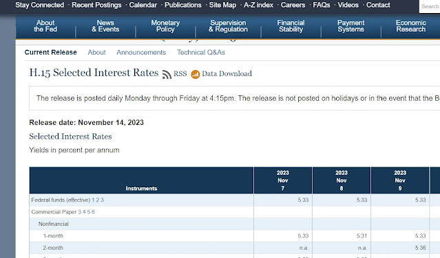
The U.S. Federal Reserve (as well as most other developed central banks) publishes a table of constant maturity yield series daily — the H.15 report. That is, for differing types of fixed income instruments (like nonfinancial commercial paper), there are rates posted by maturity (1-month, 2-month, etc.). These maturities are clean time frames, not things like “9 years, 7 months, and 3 days” if you had to use issued securities. (Swaps are naturally clean maturities since the benchmark tenors are the ones usually quoted.)
Depending on the source, there are different ways of calculating a constant maturity series.
-
Just use the yield of the benchmark bond at that maturity. The problem with this is that the yield jumps when we switch to a new benchmark.
-
Fit a yield curve through all bonds, then read off the fitted curve at that maturity. (My preference, but you can get benchmark effects, and the fitted curve can be quite different than the benchmark yield, which gets some people mad.)
-
Fit based on bonds in that maturity bucket (which the Fed H.15 uses), which keeps the fit closer to the benchmark yield.
The yield quotes can be thought of as corresponding to the yield on a par coupon bond (link to primer on par coupon bonds). As quick summary, a par coupon bond is bond whose yield matches the coupon rate — which has the effect that the bond price is at par. E.g., if the par coupon rate for the 10-year yield is 4%, then a 10-year bond with a coupon of 4% will have a price of $100 (and a yield of 4%).
So How Do You Lose Money?
Although government bonds are often described as “risk free,” that really refers to credit risk free — floating currency sovereigns are effectively immune to involuntary default for financial reasons. (Some people disagree with that assessment, but they are incorrect.) Although payments are guaranteed, you still face potential capital losses on the bond ahead of maturity.
As a reminder, yield up → price down, and vice-versa. When you buy a bond, you can calculate the internal rate of return from the payments based on the initial payment price, and modulo some fixed income yield conventions, that is the quoted yield that corresponds to that price. Easiest way to see how it works is to play with the bond price function that is typically built in to spreadsheet software.
If bond yields rise after you bought the bond, this implies a higher discount rate, and thus the corresponding price for the bond drops.
The proper way to calculate returns is with some bond pricing routines. However, we can approximate the return on holding a bond by:
Return = (interest earned over the period — “carry”) + (change in yield)×(modified duration).
The first component is relatively straightforward — just multiply the starting yield by the fraction of a year that the holding period represents. This is a bit annoying for daily calculations (since the holding period changes between weekends, weekdays, and around holidays). There is an issue regarding the reality that bond yield quotes follow funny conventions, but just dividing the yield by 12 for a monthly holding period is going to be a “good enough” approximation in most cases.
The second term is trickier. There are a few variants of “duration” used in fixed income (and show up in bond fund published statistics), but modified duration (or effective duration, which is the same thing as modified duration for option-free government bonds) is the first order sensitivity of bond returns to changes in yield (that is, the first term to the Taylor series of capital gains as a function of yield). Note that this is an approximation since the modified duration changes as yield changes — so we need higher order terms to calculate the returns properly for large yield changes.
As noted, the modified duration depends upon the bond yield and its characteristics (maturity, coupon), but is generally below the maturity in years (decreasing as yields increase). At the time of writing, the benchmark 10-year Treasury has an effective duration of 7.91. (the S&P U.S. Treasury Bond Current 10-Year Index is an index that tracks the 10-year benchmark). The approximation suggests that we would lose 7.91% if the 10-year yield rose by 1% (100 basis points). However, the losses would be less for such a large move — the second order term of the Taylor series (“convexity”) would reduce the loss. Nevertheless, it would still be enough to wipe out more than a year of income.

I will then just leave the exercise of eyeballing the yield changes on the H.15 10-year Treasury yield chart above to get an idea how much money hapless longs lost since 2020. (The S&P index previously linked gives a more precise view.)
Calculating Returns With the H.15 Data
It is a fairly standard exercise to calculate total returns for bonds based on central bank constant maturity yield data using the formula above. (One reason to do this is that bond index data is normally quite expensive — only a handful of deep-pocketed investors are really interested in the data.) If one properly accounts for the change in duration as yields change (simplest version is to take the average of start and end duration for each period), the results are going to be close to an index return (which abstracts away from transaction costs). However, there will be some unavoidable gaps due to missing security-level data.
-
As a new benchmark bond is issued, it typically trades expensive relative to bonds issued earlier. If the “constant maturity” series just uses the benchmark yield, then there will be a change in yields due to the benchmark change that does not correspond to yield changes for other bonds. If the constant maturity uses a fitting procedure, this effect is smaller but still present. Since this effect is happening every benchmark change and the error is the same direction, the error will accumulate over time, with the return proxy being lower than index returns.
-
There is normally a slope to the curve. For example, one might have a period where the 9-year yield is consistently 20 basis points lower than the 10-year. This means that bond yields “roll down” the curve, and there will be roughly 20 basis points per year of capital gains missed if one just looks at the 10-year point.
-
Benchmarks often have advantageous funding rates in the repo market. Although this matters to investors with access to the repo market, index calculations will ignore this effect.
We cannot infer the size of these effects from just the constant maturity yield data, but they generally result in the approximate returns being below index returns. However, if one is comparing returns to other asset classes (equities, cash), these calculation defects are not that significant versus the wide returns spreads between asset classes. They would matter more if one is doing a long-term returns comparison.

